Lab 3 - Tessellations, Point-in-Polygon

Authors

Completed by: Colleen Hoskins

Created by: Mike Johnson, PhD

In this lab we will an explore the impacts of tessellated surfaces and the modifiable areal unit problem (MAUP) using the National Dam Inventory maintained by the United States Army Corps of Engineers. Doing this will require repetitive tasks that we will write as functions and careful consideration of feature aggregation/simplification, spatial joins, and data visualization. The end goal is to visualize the distribution of dams and there purposes across the country.

DISCLAIMER: This lab will be crunching a TON of data, in some cases 562,590,604 values for a single process! Therefore, I encourage you to run your code chuck-by-chunk rather then regularly knitting. Your final knit may take a couple of minutes to process. I know this is painful but be proud that, all said, your report will be analyzing billions of meaningful data and geometric relations.

libraries:

library(tidyverse)
library(sf)
library(AOI)
library(mapview)
library(rmapshaper)
library(knitr)
library(kableExtra)
library(rmarkdown)
library(ggplot2)
library(units)
library(gghighlight)
library(leaflet)
library(leafem)
library(glue)

Question 1:

Here we will prepare five tessellated surfaces from CONUS and write a function to plot them in a descriptive way.

Step 1.1

First, we need a spatial file of CONUS counties. For future area calculations we want these in an equal area projection (EPSG:5070).

To achieve this:

get an sf object of US counties (AOI::aoi_get(state = “conus”, county = “all”))
transform the data to EPSG:5070

conus <- AOI::aoi_get(state = "conus", county = "all") %>%
  st_transform(crs = 5070)

Step 1.2

For triangle based tessellations we need point locations to serve as our “anchors”.

To achieve this:

generate county centroids using st_centroid
Since, we can only tessellate over a feature we need to combine or union the resulting 3,108 POINT features into a single MULTIPOINT feature
Since these are point objects, the difference between union/combine is mute

centroid <- conus %>%
  st_centroid() %>%
  st_combine()

Step 1.3

Make a voronoi tessellation over your county centroids (MULTIPOINT)

voronoi <- st_voronoi(centroid, envelope = st_union(conus)) %>%
  st_collection_extract("POLYGON") %>%
  st_as_sf() %>%
  mutate(id = row_number()) %>%
  st_cast()

Make a triangulated tessellation over your county centroids (MULTIPOINT)

triangulated <- st_triangulate(centroid) %>%
  st_collection_extract("POLYGON") %>%
  st_as_sf() %>%
  mutate(id = row_number()) %>%
  st_cast()

Make a gridded coverage with n = 70, over your counties object

grid <- st_make_grid(conus, n = 70, what = "polygons", square = TRUE) %>%
  st_as_sf() %>%
  mutate(id = row_number ()) %>%
  st_cast()

Make a hexagonal coverage with n = 70, over your counties object In addition to creating these 4 coverage’s we need to add an ID to each tile.

hex <- st_make_grid(conus, n = 70, what = "polygons", square = FALSE) %>%
  st_as_sf() %>%
  mutate(id = row_number ()) %>%
  st_cast()

Step 1.4

If you plot the above tessellations you’ll see the triangulated surfaces produce regions far beyond the boundaries of CONUS.

We need to cut these boundaries to CONUS border.

To do this, we will call on st_intersection, but will first need a geometry of CONUS to serve as our differencing feature. We can get this by unioning our existing county boundaries.

union <- st_union(conus) 

voronoi_union <- st_intersection(voronoi, union)

triangulated_union <- st_intersection(triangulated, union)

grid_union <- st_intersection(grid, union)

hex_union <- st_intersection(hex, union)

Step 1.5

With a single feature boundary, we must carefully consider the complexity of the geometry. Remember, the more points our geometry contains, the more computations needed for spatial predicates our differencing. For a task like ours, we do not need a finely resolved coastal boarder.

To achieve this:

Simplify your unioned border using the Visvalingam algorithm provided by rmapshaper::ms_simplify.
Choose what percentage of vertices to retain using the keep argument and work to find the highest number that provides a shape you are comfortable with for the analysis:

simple <- ms_simplify(
  union,
  keep = .05, 
  method = "vis",
  weighting = 0.7,
  keep_shapes = FALSE,
  no_repair = FALSE,
  snap = TRUE,
  explode = FALSE,
  drop_null_geometries = TRUE,
  snap_interval = NULL)

Once you are happy with your simplification, use the mapview::npts function to report the number of points in your original object, and the number of points in your simplified object.

mapview::npts(union)

[1] 11292

mapview::npts(simple)

[1] 577

How many points were you able to remove? What are the consequences of doing this computationally?
- 10,715 points. This will make computation faster but we will lose detail.
Finally, use your simplified object to crop the two triangulated tessellations with st_intersection:

voronoi_simple <- st_intersection(voronoi, simple)
triangulated_simple <- st_intersection(triangulated, simple)

Step 1.6

The last step is to plot your tessellations. We don’t want to write out 5 ggplots (or mindlessly copy and paste 😄)

Instead, lets make a function that takes an sf object as arg1 and a character string as arg2 and returns a ggplot object showing arg1 titled with arg2.

For this function:

The name can be anything you chose, arg1 should take an sf object, and arg2 should take a character string that will title the plot
In your function, the code should follow our standard ggplot practice where your data is arg1, and your title is arg2
The function should also enforce the following:
- a white fill
- a navy border
- a size of 0.2
- `theme_void``
- a caption that reports the number of features in arg1
You will need to paste character stings and variables together.

tess_plot = function(object, title_text) {
  ggplot(data = object) +
  geom_sf(fill = "white", color = "navy", size = 0.2) +
  theme_void() +
  labs(
    title = title_text,
    caption = paste("number of features:", nrow(object)))
}

tess_plot(voronoi_simple, "voronoi plot")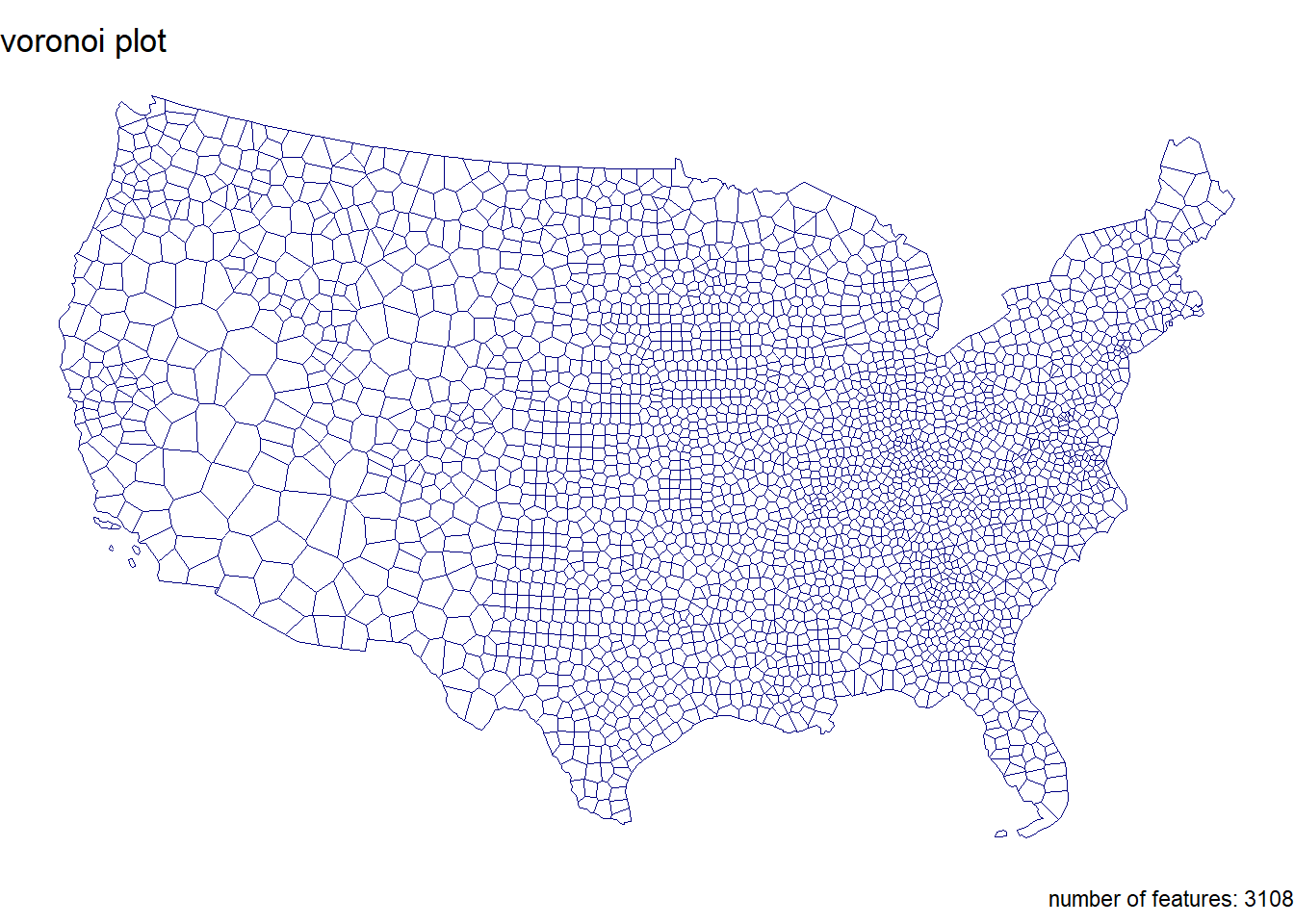

Step 1.7

Use your new function to plot each of your tessellated surfaces and the original county data (5 plots in total):

tess_plot(conus, "CONUS County Boundaries")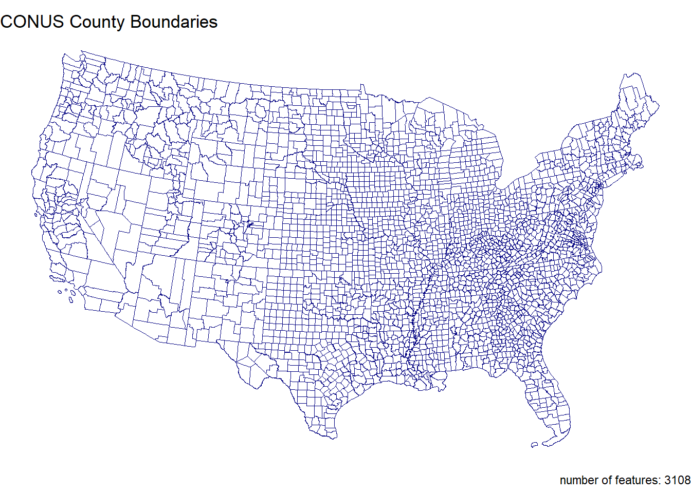

tess_plot(voronoi_simple, "Voronoi Tessellation")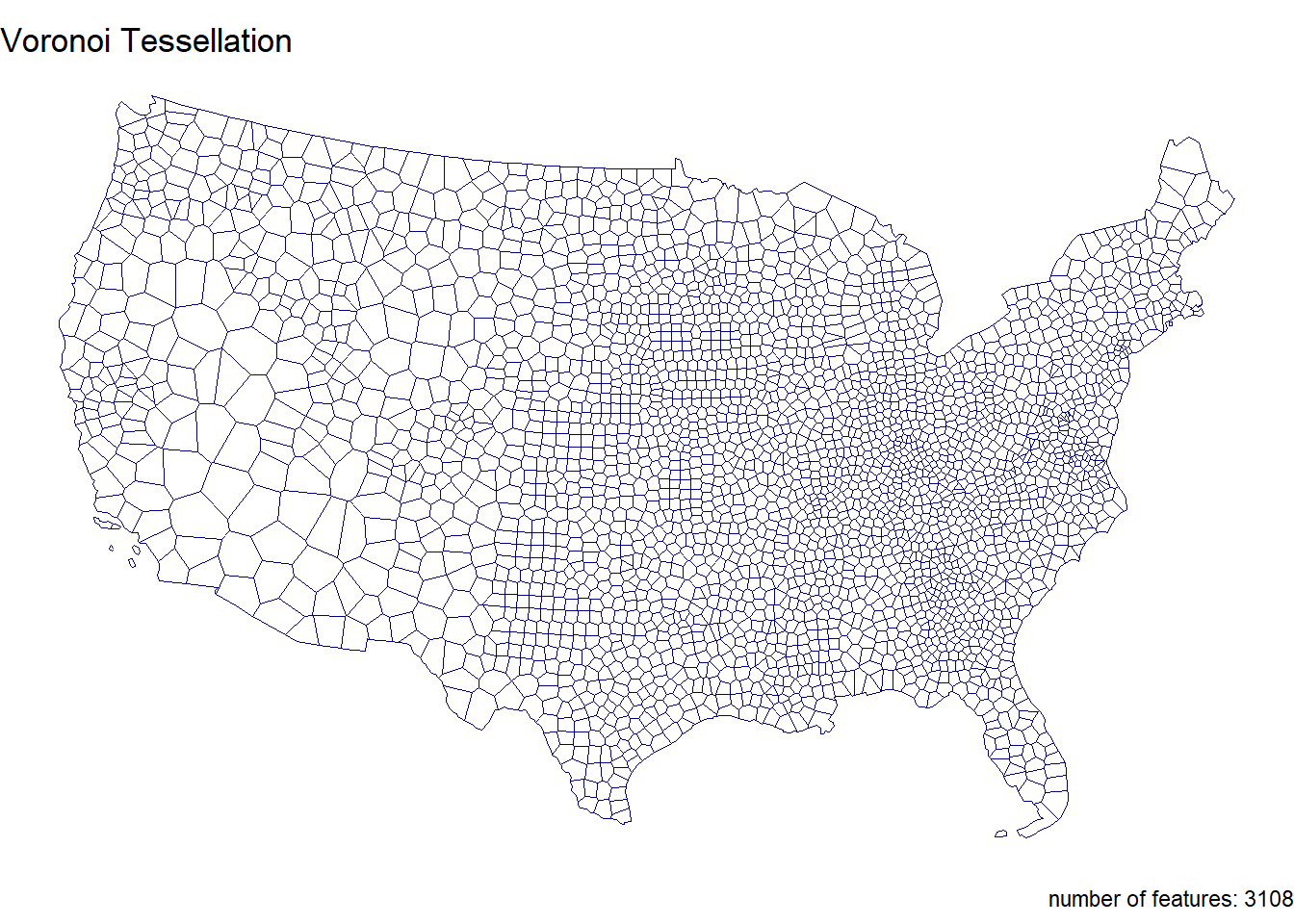

tess_plot(triangulated_simple, "Triangulated Tessellation")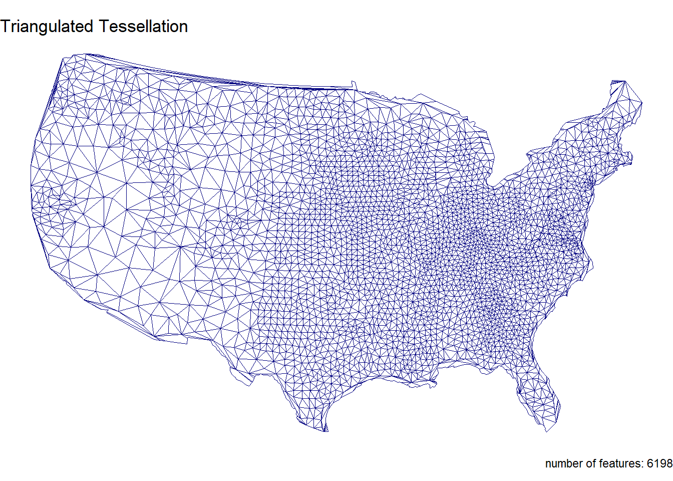

tess_plot(grid_union, "Square Grid Tessellation")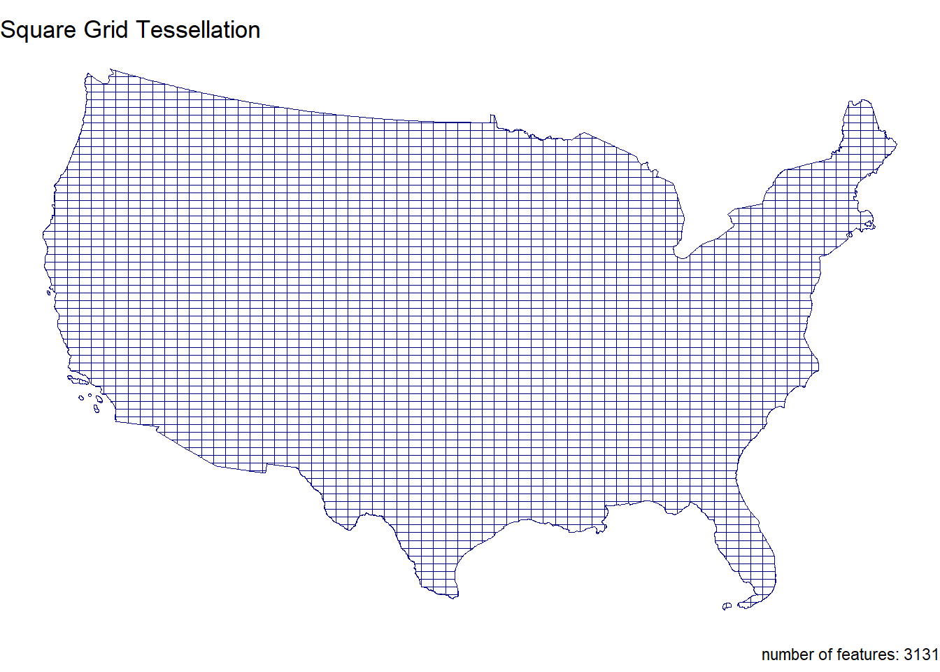

tess_plot(hex_union, "Hexagonal Grid Tessellation")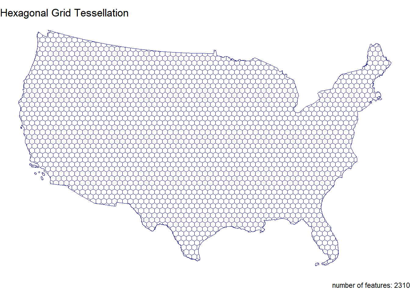

Question 2

In this question, we will write out a function to summarize our tessellated surfaces. Most of this should have been done in your daily assignments.

Step 2.1

First, we need a function that takes a sf object and a character string and returns a data.frame.

For this function:

The function name can be anything you chose, arg1 should take an sf object, and arg2 should take a character string describing the object
In your function, calculate the area of arg1; convert the units to km2; and then drop the units
Next, create a data.frame containing the following:
- text from arg2
- the number of features in arg1
- the mean area of the features in arg1 (km2)
- the standard deviation of the features in arg1
- the total area (km2) of arg1
Return this data.frame

tess_sum <- function(sf_object, character_string) {
  
  area_m2 <- st_area(sf_object)
  
  area_km2 <- set_units(area_m2, "km^2") %>%
    as.numeric()
  
  data.frame(
    description = character_string,
    num_features = length(area_km2),
    mean_area_km2 = mean(area_km2),
    sd_area_km2 = sd(area_km2),
    total_area_km2 = sum(area_km2)
  )
}

Step 2.2

Use your new function to summarize each of your tessellations and the original counties.

conus_sum <- tess_sum(conus, "CONUS")
conus_sum

  description num_features mean_area_km2 sd_area_km2 total_area_km2
1       CONUS         3108       2605.05    3443.712        8096496

voronoi_sum <- tess_sum(voronoi_simple, "Voronoi Tessallation")
voronoi_sum

           description num_features mean_area_km2 sd_area_km2 total_area_km2
1 Voronoi Tessallation         3108      2604.426    2917.817        8094557

triangulated_sum <- tess_sum(triangulated_simple, "Triangulated Tessellation")
triangulated_sum

                description num_features mean_area_km2 sd_area_km2
1 Triangulated Tessellation         6198      1290.368    1598.403
  total_area_km2
1        7997700

grid_sum <- tess_sum(grid_union, "Square Grid Tessellation")
grid_sum

               description num_features mean_area_km2 sd_area_km2
1 Square Grid Tessellation         3131      2585.914      572.79
  total_area_km2
1        8096496

hex_sum <- tess_sum(hex_union, "Hexagonal Grid Tessellation")
hex_sum

                  description num_features mean_area_km2 sd_area_km2
1 Hexagonal Grid Tessellation         2310      3504.976    839.2546
  total_area_km2
1        8096496

Step 2.3

Multiple data.frame objects can bound row-wise with bind_rows into a single data.frame

sum_all <- bind_rows(
  conus_sum,
  voronoi_sum,
  triangulated_sum,
  grid_sum,
  hex_sum
)

sum_all <- sum_all %>%
  rename(
    Description = description,
    `Number of Features` = num_features,
    `Mean Area (km²)` = mean_area_km2,
    `SD Area (km²)` = sd_area_km2,
    `Total Area (km²)` = total_area_km2
  )

Step 2.4

Once your 5 summaries are bound (2 tessellations, 2 coverage’s, and the raw counties) print the data.frame as a nice table using knitr/kableExtra.

sum_all %>%
  kable(format = "html", caption = "Comparison of Spatial Coverages and Tessellations", digits = 2) %>%
  kable_styling(full_width = FALSE, bootstrap_options = c("striped", "hover", "condensed", "responsive"))

Comparison of Spatial Coverages and Tessellations
Description	Number of Features	Mean Area (km²)	SD Area (km²)	Total Area (km²)
CONUS	3108	2605.05	3443.71	8096496
Voronoi Tessallation	3108	2604.43	2917.82	8094557
Triangulated Tessellation	6198	1290.37	1598.40	7997700
Square Grid Tessellation	3131	2585.91	572.79	8096496
Hexagonal Grid Tessellation	2310	3504.98	839.25	8096496

Step 2.5 Comment on the traits of each tessellation. Be specific about how these traits might impact the results of a point-in-polygon analysis in the contexts of the modifiable areal unit problem and with respect computational requirements.

Voronoi and triangulated tessellations are sensitive to the Modifiable Areal Unit Problem (MAUP), as the shape and size of their polygons depend on centroid placement, potentially misaligning with natural boundaries. Grid tessellations are less affected by MAUP but may misalign with natural features, while hexagonal tessellations offer a more uniform and less biased representation. Computationally, grid and hexagonal tessellations are more efficient than Voronoi and triangulated tessellations, which require more complex geometric calculations.

Question 3:

The data we are going to analysis in this lab is from US Army Corp of Engineers National Dam Inventory (NID). This dataset documents ~91,000 dams in the United States and a variety of attribute information including design specifications, risk level, age, and purpose.

For the remainder of this lab we will analysis the distributions of these dams (Q3) and their purpose (Q4) through using a point-in-polygon analysis.

Step 3.1

In the tradition of this class - and true to data science/GIS work - you need to find, download, and manage raw data. While the raw NID data is no longer easy to get with the transition of the USACE services to ESRI Features Services, I staged the data in the resources directory of this class. To get it, navigate to that location and download the raw file into you lab data directory.

Return to your RStudio Project and read the data in using the readr::read_csv
After reading the data in, be sure to remove rows that don’t have location values (!is.na())
Convert the data.frame to a sf object by defining the coordinates and CRS
Transform the data to a CONUS AEA (EPSG:5070) projection - matching your tessellation
Filter to include only those within your CONUS boundary

dams = readr::read_csv('data/NID2019_U.csv') 

usa <- AOI::aoi_get(state = "conus") %>% 
  st_union() %>% 
  st_transform(5070)

dams2 = dams %>% 
  filter(!is.na(LATITUDE) ) %>%
  st_as_sf(coords = c("LONGITUDE", "LATITUDE"), crs = 4236) %>% 
  st_transform(5070) %>% 
  st_filter(usa)

Step 3.2

Step 3.2 Following the in-class examples develop an efficient point-in-polygon function that takes:

points as arg1,
polygons as arg2,
The name of the id column as arg3

The function should make use of spatial and non-spatial joins, sf coercion and dplyr::count. The returned object should be input sf object with a column - n - counting the number of points in each tile.

point_poly <- function(points, polygons, id) {
  joined <- st_join(points, polygons[id], left = FALSE)
  
  counts <- joined %>%
    st_drop_geometry() %>%
    count(!!sym(id), name = "n")
  
  polygons %>%
    left_join(counts, by = id) %>%
    mutate(n = ifelse(is.na(n), 0, n))
}

Step 3.3

Apply your point-in-polygon function to each of your five tessellated surfaces where:

Your points are the dams
Your polygons are the respective tessellation
The id column is the name of the id columns you defined

dams_conus <- point_poly(dams2, conus, "fip_code")
dams_voronoi <- point_poly(dams2, voronoi_simple, "id")
dams_triangulated <- point_poly(dams2, triangulated_simple, "id")
dams_grid <- point_poly(dams2, grid_union, "id")
dams_hex <- point_poly(dams2, hex_union, "id")

Step 3.4

Lets continue the trend of automating our repetitive tasks through function creation. This time make a new function that extends your previous plotting function.

For this function:

The name can be anything you chose, arg1 should take an sf object, and arg2 should take a character string that will title the plot
The function should also enforce the following:
- the fill aesthetic is driven by the count column n
- the col is NA
- the fill is scaled to a continuous viridis color ramp
- theme_void
- a caption that reports the number of dams in arg1 (e.g. sum(n))
  - You will need to paste character strings and variables together.

dam_plot <- function(object, title_text) {
  object <- object %>%
    filter(st_geometry_type(.) %in% c("POLYGON", "MULTIPOLYGON")) %>%
    filter(!st_is_empty(.)) %>%
    filter(st_is_valid(.)) %>%
    filter(!is.na(n)) %>%
    mutate(n = as.numeric(n))

  ggplot(data = object) +
    geom_sf(aes(fill = n), color = NA) +
    scale_fill_viridis_c(option = "viridis", na.value = "white") +
    theme_void() +
    labs(
      title = title_text,
      caption = paste("total number of dams:", sum(object$n, na.rm = TRUE)),
      fill = "dam count"
    )
}

Step 3.5

Apply your plotting function to each of the 5 tessellated surfaces with Point-in-Polygon counts:

dam_plot(dams_conus, "County")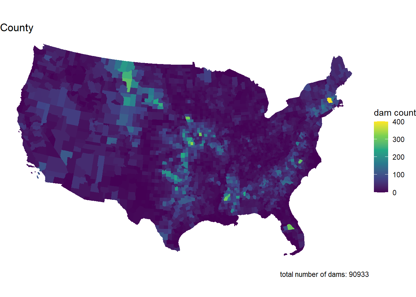

dam_plot(dams_voronoi, "Voronoi Tessellation")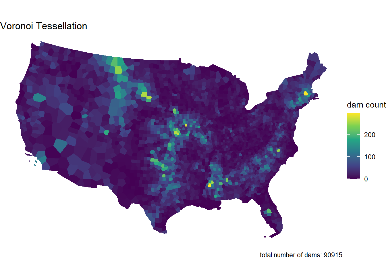

dam_plot(dams_triangulated, "Triangulated Tessellation")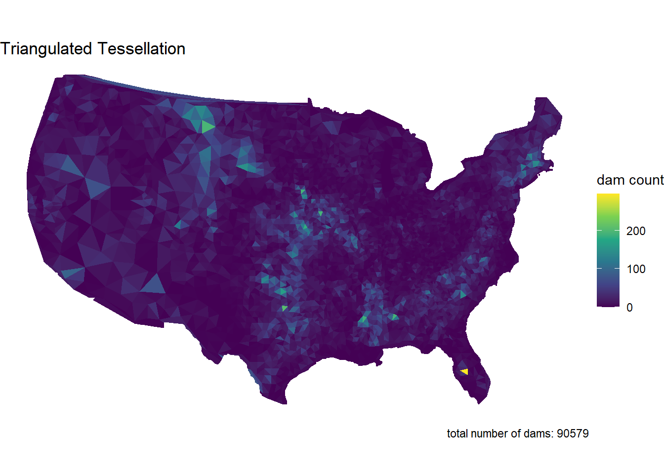

dam_plot(dams_grid, "Square Grid")

dam_plot(dams_hex, "Hexagonal Grid")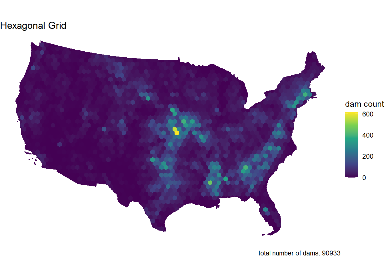

Step 3.6

Comment on the influence of the tessellated surface in the visualization of point counts. How does this related to the MAUP problem. Moving forward you will only use one tessellation, which will you chose and why?

I’m choosing the hexagonal grid tessellation because it gives a more even and balanced view of point counts, making it easier to see concentration areas without the distortion you might get with Voronoi or triangulated tessellations. The uniform shape helps avoid the issues of the Modifiable Areal Unit Problem (MAUP), which can mess with analysis when shapes vary too much. It also works well for visualizing the concentration in the Midwest and South, and it’s more computationally efficient for larger datasets.

Question 4

Step 4.1

Your task is to create point-in-polygon counts for at least 4 of the follwing dam purposes:
- I Irrigation
- H Hydroelectric
- C Flood Control
- N Navigation
- S Water Supply
- R Recreation
- P Fire Protection
- F Fish and Wildlife
- D Debris Control
- T Tailings
- G Grade Stabilization
- O Other
You will use grepl to filter the complete dataset to those with your chosen purpose
Remember that grepl returns a boolean if a given pattern is matched in a string
grepl is vectorized so can be used in dplyr::filter

For your analysis, choose at least four of the above codes, and describe why you chose them. Then for each of them, create a subset of dams that serve that purpose using dplyr::filter and grepl

I chose Irrigation, Hydroelectric, Flood Control, and Water Supply. I chose these because they are uses for dams that I am most familiar with.

Finally, use your point-in-polygon function to count each subset across your elected tessellation

dams_i <- dams2 %>%
  filter(grepl("I", PURPOSES))

dams_h <- dams2 %>%
  filter(grepl("H", PURPOSES))

dams_c <- dams2 %>%
  filter(grepl("C", PURPOSES))

dams_s <- dams2 %>%
  filter(grepl("S", PURPOSES))

dams_i_hex <- point_poly(dams_i, hex_union, "id")
dams_h_hex <- point_poly(dams_h, hex_union, "id")
dams_c_hex <- point_poly(dams_c, hex_union, "id")
dams_s_hex <- point_poly(dams_s, hex_union, "id")

Step 4.2

Now use your plotting function from Q3 to map these counts.
But! you will use gghighlight to only color those tiles where the count (n) is greater then the (mean + 1 standard deviation) of the set
Since your plotting function returns a ggplot object already, the gghighlight call can be added “+” directly to the function.
The result of this exploration is to highlight the areas of the country with the most

mean_sd_i <- mean(dams_i_hex$n) + sd(dams_i_hex$n)
mean_sd_h <- mean(dams_h_hex$n) + sd(dams_h_hex$n)
mean_sd_c <- mean(dams_c_hex$n) + sd(dams_c_hex$n)
mean_sd_s <- mean(dams_s_hex$n) + sd(dams_s_hex$n)

dam_plot(dams_i_hex, "Irrigation Dams") +
  gghighlight(n > mean_sd_i, label_key = n)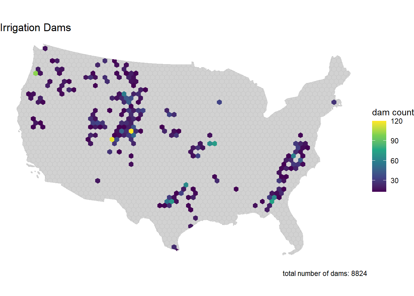

dam_plot(dams_h_hex, "Hydroelectric Dams") +
  gghighlight(n > mean_sd_h, label_key = n)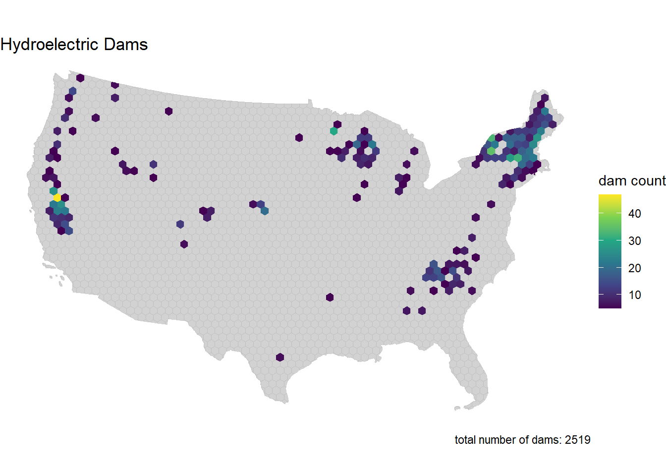

dam_plot(dams_c_hex, "Flood Control Dams") +
  gghighlight(n > mean_sd_c, label_key = n)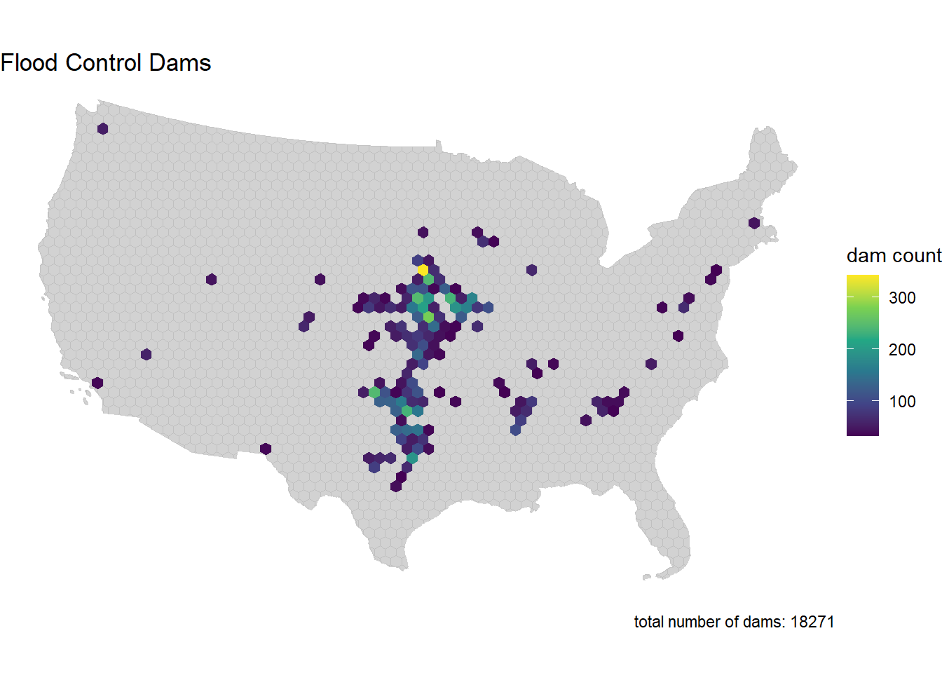

dam_plot(dams_s_hex, "Water Supply Dams") +
  gghighlight(n > mean_sd_s, label_key = n)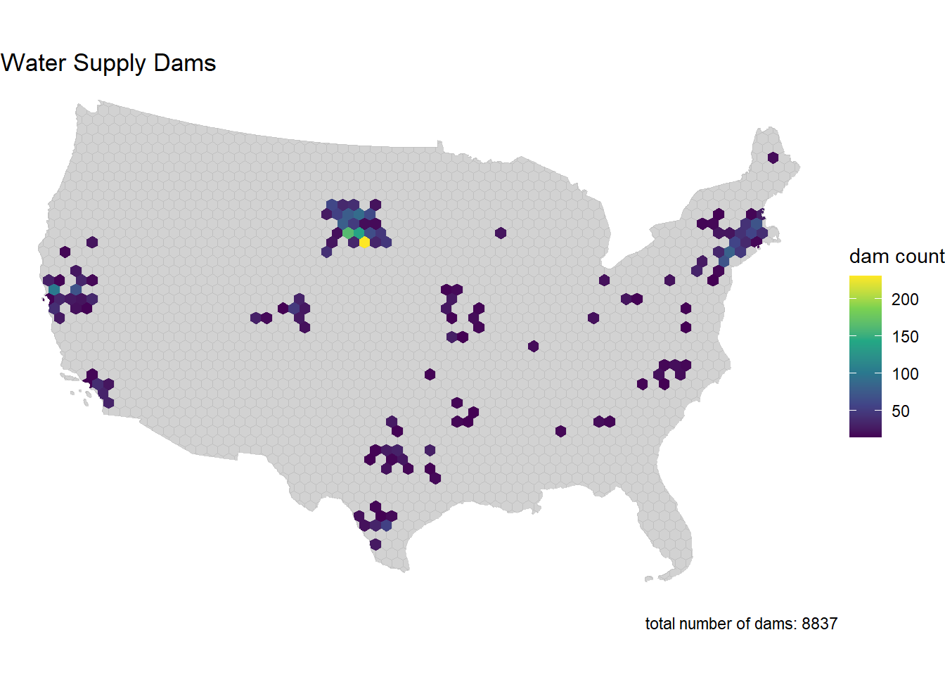

Step 4.3

Comment of geographic distribution of dams you found. Does it make sense? How might the tessellation you chose impact your findings? How does the distribution of dams coincide with other geographic factors such as river systems, climate, ect?

Irrigation dams are most concentrated around what looks like Wyoming, Utah, Colorado and Texas. That makes sense, as these areas divert water for irrigation. Hydroelectric dams are concentrated in the Northeast and West Coast. This makes sense, as the states that produce the most hydropower are Washington, New York, California, and Oregon. Flood Control dams are concentrated around the Midwest and seem to be in areas that the Mississippi River runs through. Finally, water supply dams are scattered. They may represent areas with high population or with high agricultural water needs.

Question 5:

You have also been asked to identify the largest, at risk, flood control dams in the country

You must also map the Mississippi River System - This data is available here - Download the shapefile and unzip it into your data directory. - Use read_sf to import this data and filter it to only include the Mississippi SYSTEM

To achieve this:

Create an interactive map using leaflet to show the largest (NID_STORAGE); high-hazard (HAZARD == “H”) dam in each state

The markers should be drawn as opaque, circle markers, filled red with no border, and a radius set equal to the (NID_Storage / 1,500,000)
The map tiles should be selected from any of the tile providers
A popup table should be added using leafem::popup and should only include the dam name, storage, purposes, and year completed
The Mississippi system should be added at a Polyline feature

major_rivers <- read_sf("data/major_rivers/MajorRivers.shp")

miss <- major_rivers %>%
  filter(SYSTEM == "Mississippi") %>%
  st_transform(crs = 4326)

H <- dams2 %>%
  mutate(STATE_CODE = substr(NIDID, 1, 2)) %>%
  filter(HAZARD == "H", grepl("C", PURPOSES)) %>%
  group_by(STATE_CODE) %>%
  slice_max(order_by = NID_STORAGE, n = 1, with_ties = FALSE) %>%
  ungroup() %>%
  st_transform(crs = 4326)

H$popup <- glue::glue_data(
  H,
  "<b>{DAM_NAME}</b><br/>",
  "Storage: {format(NID_STORAGE, big.mark = ',')} acre-ft<br/>",
  "Purposes: {PURPOSES}<br/>",
  "Year Completed: {YEAR_COMPLETED}"
)


leaflet() %>%
  addProviderTiles("CartoDB.Positron") %>%
  addPolylines(data = miss, color = "blue", weight = 2, opacity = 0.8) %>%
  addCircleMarkers(
    data = H,
    radius = ~NID_STORAGE / 1500000,
    color = NA,
    fillColor = "red",
    fillOpacity = 0.8,
    label = ~DAM_NAME,
    popup = ~popup
  )